Bias Variance Dilemma
I will be publishing the homeworks that I have done for Pattern Recognition course, I believe that they deal with important topics in Pattern Recognition and someone may benefit from them.
For anyone that needs to get deep in the theory of Pattern Recognition and train themselves in the field I suggest our course book Introduction to Machine Learning by Ethem Alpaydin.
A quite general phenomenon arising in all kinds of pattern recognition methods is the dilemma between bias and variance. The bias and variance we are speaking of are two properties of our model that seem to have a conflicting relation. Whenever we fit a model to a data, we can notice two properties; bias, giving us a some kind of measure on our model’s predictions’ average closeness to training data and variance, deviation of the predictions by our model from the original data. If we fit a model with a low complexity (i.e. less assumptions), our model’s predictions on data are usually very different from real values, do not follow the real trend in data and our model introduces high bias in its predictions and because of this high bias our model will not be able to follow the real trend in data and will produce predictions that are closer to our other predictions hence low variance. As we increase the complexity, bias of our model will decrease producing much better results on prediction however our predictions will be based more strongly on our input and we will be able to fit to individual points better but a prediction will deviate more from our other predictions, increasing variance.These contrasting trends for bias and variance is the cause for bias/variance dilemma. One may question why it is called a dilemma noting that our predictions get better with more complexity and model with the highest complexity is the choice for best performance. However, we should never lose sight of the fact that we are fitting a model to the available data and actually only performance on training data is getting better. As we increase the complexity of our models, there is a critical point where our model performs best on data that it is not trained on (test data). This point corresponds to the point where sum of bias and variance for our model reaches a minimum.
In this post, we will aim to observe the bias/variance dilemma in the context of polynomial regression. We will a generate a synthetic training data by producing samples by taking points on a known function and adding a random normal noise to them. Our input function: f(x)=2sin(1.5x) where x is uniform between 0 and 5 We will add random normal noise with mean 0 and standard deviation 1. We will generate 100 samples each containing i=1,…,20 points sampled as above. We will also generate a separate validation set containing 100 points without noise.
We will fit polynomials of degree 1 to 5 to training data and calculate their bias and variances.
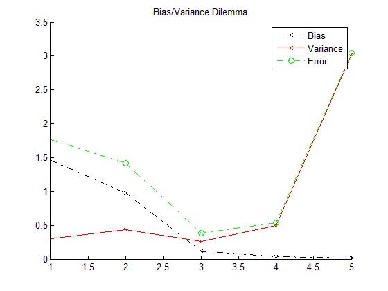
As it can be seen from the above plot, bias of the estimator decreases with degree of the polynomial fitted while variance of the estimator increases. For every different sample, when the polynomial degree increases, the polynomials fit to samples with less error. However, since the data is taken from a noisy training set, this also means that the fitted polynomials also learn the error which harms the flexibility and estimation power of the fitted models. Average fits get closer to actual function as the degree increases and the bias of models presents a declining trend. However, variance of models rises due to the fact that polynomials also learn the noise in the data set. Total error which is the sum of bias2 and variance reaches a minimum at degree 3 which is optimal degree for the given problem. For degrees under 3, model under-fits the data while for larger degrees it over-fits.
1
2
3
4
5
6
7
8
9
10
11
12
13
14
15
16
17
18
19
20
21
22
23
24
25
26
27
28
29
30
31
32
33
34
35
36
37
38
39
40
41
42
43
44
45
46
47
48
49
50
51
52
53
54
55
56
57
58
59
60
61
62
63
64
65
66
67
68
69
70
71
72
73
74
75
76
77
78
79
80
81
82
83
84
85
86
87
88
89
90
91
92
93
94
95
96
97
98
99
100
101
102
103
104
105
106
107
108
109
110
111
112
113
114
115
% This program is free software: you can redistribute it and/or modify
% it under the terms of the GNU General Public License as published by
% the Free Software Foundation, either version 3 of the License, or
% (at your option) any later version.
%
% This program is distributed in the hope that it will be useful,
% but WITHOUT ANY WARRANTY; without even the implied warranty of
% MERCHANTABILITY or FITNESS FOR A PARTICULAR PURPOSE.  See the
% GNU General Public License for more details.
%
% You should have received a copy of the GNU General Public License
% along with this program.  If not, see http://www.gnu.org/licenses/

x = zeros(100,20); %initialize training set inputs
r = zeros(100,20); %initialize training set outputs
for i = 1:1:100 %create 100 samples with 20 points each
    x(i,:) = sort(rand(1,20)*5); %sort the input that plot can draw the lines between points
    r(i,:) = 2*sin(1.5*x(i,:)) + randn(1,20); %calculate training set outputs
end

xv = sort(rand(1,100)*5); %validation set inputs
rv = 2*sin(1.5*xv); %validation set outputs

%create matrices for holding equation coefficients
coeffs1 = zeros(100,2); % 1st degree
coeffs2 = zeros(100,3); % 2st degree
coeffs3 = zeros(100,4); % 3st degree
coeffs4 = zeros(100,5); % 4st degree
coeffs5 = zeros(100,6); % 5st degree
for i = 1:1:100         % calculate coefficients for each sample set
    coeffs1(i,:) = polyfit(x(i,:),r(i,:),1);    % fit a 1st degree polynomial to ith sample
    coeffs2(i,:) = polyfit(x(i,:),r(i,:),2);    % fit a 2st degree polynomial to ith sample
    coeffs3(i,:) = polyfit(x(i,:),r(i,:),3);    % fit a 3st degree polynomial to ith sample
    coeffs4(i,:) = polyfit(x(i,:),r(i,:),4);    % fit a 4st degree polynomial to ith sample
    coeffs5(i,:) = polyfit(x(i,:),r(i,:),5);    % fit a 5st degree polynomial to ith sample
end
avgcoeff1 = sum(coeffs1)/100;   % calculate average 1st degree equation coefficients
avgcoeff2 = sum(coeffs2)/100;   % calculate average 2st degree equation coefficients
avgcoeff3 = sum(coeffs3)/100;   % calculate average 3st degree equation coefficients
avgcoeff4 = sum(coeffs4)/100;   % calculate average 4st degree equation coefficients
avgcoeff5 = sum(coeffs5)/100;   % calculate average 5st degree equation coefficients

plotx = 0:0.2:5;    % x values for plotting
figure
hold on
plot(xv,rv,'-r','LineWidth',2); % plot validation set
% plot 5 different fits
plot(plotx, polyval(coeffs1(10,:),plotx),'-r');
plot(plotx, polyval(coeffs1(20,:),plotx),'-g');
plot(plotx, polyval(coeffs1(30,:),plotx),'-b');
plot(plotx, polyval(coeffs1(40,:),plotx),'-c');
plot(plotx, polyval(coeffs1(50,:),plotx),'-m');
% plot average fit
plot(plotx, polyval(avgcoeff1,plotx),'-.ok','LineWidth',2);
legend('2*sin(1.5*x)','Ex. Fit 1','Ex. Fit 2','Ex. Fit 3','Ex. Fit 4','Ex. Fit 5','Average Fit');
title('1st Degree Fits');
hold off
figure
hold on
plot(xv,rv,'-r','LineWidth',2); % plot validation set
% plot 5 different fits
plot(plotx, polyval(coeffs3(10,:),plotx),'-r');
plot(plotx, polyval(coeffs3(20,:),plotx),'-g');
plot(plotx, polyval(coeffs3(30,:),plotx),'-b');
plot(plotx, polyval(coeffs3(40,:),plotx),'-c');
plot(plotx, polyval(coeffs3(50,:),plotx),'-m');
% plot average fit
plot(plotx, polyval(avgcoeff3,plotx),'-.ok','LineWidth',2);
legend('2*sin(1.5*x)','Ex. Fit 1','Ex. Fit 2','Ex. Fit 3','Ex. Fit 4','Ex. Fit 5','Average Fit');
title('3rd Degree Fits');
hold off
figure
hold on
plot(xv,rv,'-r','LineWidth',2); % plot validation set
% plot 5 different fits
plot(plotx, polyval(coeffs5(10,:),plotx),'-r');
plot(plotx, polyval(coeffs5(20,:),plotx),'-g');
plot(plotx, polyval(coeffs5(30,:),plotx),'-b');
plot(plotx, polyval(coeffs5(40,:),plotx),'-c');
plot(plotx, polyval(coeffs5(50,:),plotx),'-m');
% plot average fit
plot(plotx, polyval(avgcoeff5,plotx),'-.ok','LineWidth',2);
legend('2*sin(1.5*x)','Ex. Fit 1','Ex. Fit 2','Ex. Fit 3','Ex. Fit 4','Ex. Fit 5','Average Fit');
title('5th Degree Fits');
hold off

% bias calculation
% sum the squared difference on validation set for each degree's average fit
bias(1) = (sum((polyval(avgcoeff1,xv)-rv).^2)) / 100;
bias(2) = (sum((polyval(avgcoeff2,xv)-rv).^2)) / 100;
bias(3) = (sum((polyval(avgcoeff3,xv)-rv).^2)) / 100;
bias(4) = (sum((polyval(avgcoeff4,xv)-rv).^2)) / 100;
bias(5) = (sum((polyval(avgcoeff5,xv)-rv).^2)) / 100;

%variance calculation
varm = zeros(100,5);
for i = 1:1:100 % calculate the variance for each sample
    % sum each fit's squared error with average fit on validation set to
    % get variances
    varm(i,1) = (sum((polyval(coeffs1(i,:),xv) - polyval(avgcoeff1,xv)).^2)) / 100;
    varm(i,2) = (sum((polyval(coeffs2(i,:),xv) - polyval(avgcoeff2,xv)).^2)) / 100;
    varm(i,3) = (sum((polyval(coeffs3(i,:),xv) - polyval(avgcoeff3,xv)).^2)) / 100;
    varm(i,4) = (sum((polyval(coeffs4(i,:),xv) - polyval(avgcoeff4,xv)).^2)) / 100;
    varm(i,5) = (sum((polyval(coeffs5(i,:),xv) - polyval(avgcoeff5,xv)).^2)) / 100;
end
vars = sum(varm)/100;   % sum sample variances to get variances for each degree
figure
hold on
% plot biases, variances and error
plot(bias,'-.xk');
plot(vars,'-xr');
plot(bias+vars,'-.og');
legend('Bias','Variance','Error');
title('Bias/Variance Dilemma');
hold off