Reparameterization Trick
Note: The IPython notebook for this post can be seen here.
Here we will try to understand the reparameterization trick used by Kingma and Welling (2014)1 to train their variational autoencoder.
Assume we have a normal distribution \(q\) that is parameterized by \(\theta\), specifically \(q_{\theta}(x) = N(\theta,1)\). We want to solve the below problem
\[\text{min}_{\theta} \quad E_q[x^2]\]This is of course a rather silly problem and the optimal \(\theta\) is obvious. But here we just want to understand how the reparameterization trick helps in calculating the gradient of this objective \(E_q[x^2]\).
The usual way to calculate \(\nabla_{\theta} E_q[x^2]\) is as follows
\[\nabla_{\theta} E_q[x^2] = \nabla_{\theta} \int q_{\theta}(x) x^2 dx = \int x^2 \nabla_{\theta} q_{\theta}(x) \frac{q_{\theta}(x)}{q_{\theta}(x)} dx = \int q_{\theta} \nabla_{\theta} \log q_{\theta}(x) x^2 dx = E_q[x^2 \nabla_{\theta} \log q_{\theta}(x)]\]which makes use of \(\nabla_{\theta} q_{\theta} = q_{\theta} \nabla_{\theta} \log q_{\theta}\). This trick is also the basis of the REINFORCE2 algorithm used in policy gradient.
For our example where \(q_{\theta}(x) = N(\theta,1)\), this method gives
\[\nabla_{\theta} E_q[x^2] = E_q[x^2 (x-\theta)]\]Reparameterization trick is a way to rewrite the expectation so that the distribution with respect to which we take the expectation is independent of parameter \(\theta\). To achieve this, we need to make the stochastic element in \(q\) independent of \(\theta\). Hence, we write \(x\) as
\[x = \theta + \epsilon, \quad \epsilon \sim N(0,1)\]Then, we can write
\[E_q[x^2] = E_p[(\theta+\epsilon)^2]\]where \(p\) is the distribution of \(\epsilon\), i.e., \(N(0,1)\). Now we can write the derivative of \(E_q[x^2]\) as follows
\[\nabla_{\theta} E_q[x^2] = \nabla_{\theta} E_p[(\theta+\epsilon)^2] = E_p[2(\theta+\epsilon)]\]Now let us compare the variances of the two methods; we are hoping to see that the first method has high variance while reparameterization trick decreases the variance substantially.
import numpy as np
N = 1000
theta = 2.0
x = np.random.randn(N) + theta
eps = np.random.randn(N)

grad1 = lambda x: np.sum(np.square(x)*(x-theta)) / x.size
grad2 = lambda eps: np.sum(2*(theta + eps)) / x.size

print grad1(x)
print grad2(eps)
4.46239612174
4.1840532024
Let us plot the variance for different sample sizes.
Ns = [10, 100, 1000, 10000, 100000]
reps = 100

means1 = np.zeros(len(Ns))
vars1 = np.zeros(len(Ns))
means2 = np.zeros(len(Ns))
vars2 = np.zeros(len(Ns))

est1 = np.zeros(reps)
est2 = np.zeros(reps)
for i, N in enumerate(Ns):
    for r in range(reps):
        x = np.random.randn(N) + theta
        est1[r] = grad1(x)
        eps = np.random.randn(N)
        est2[r] = grad2(eps)
    means1[i] = np.mean(est1)
    means2[i] = np.mean(est2)
    vars1[i] = np.var(est1)
    vars2[i] = np.var(est2)

print means1
print means2
print
print vars1
print vars2
[ 3.8409546 3.97298803 4.03007634 3.98531095 3.99579423]
[ 3.97775271 4.00232825 3.99894536 4.00353734 3.99995899]
[ 6.45307927e+00 6.80227241e-01 8.69226368e-02 1.00489791e-02
8.62396526e-04]
[ 4.59767676e-01 4.26567475e-02 3.33699503e-03 5.17148975e-04
4.65338152e-05]
%matplotlib inline
import matplotlib.pyplot as plt

plt.plot(vars1)
plt.plot(vars2)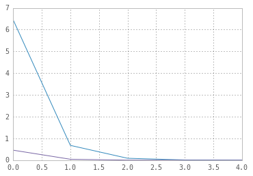
Variance of the estimates using reparameterization trick is one order of magnitude smaller than the estimates from the first method!