Variational Autoencoder
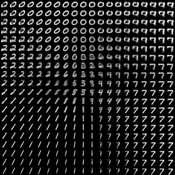
I have recently implemented the variational autoencoder proposed in Kingma and Welling (2014)1. This is a rather interesting unsupervised learning model. In contrast to most earlier work, Kingma and Welling (2014)1 optimize the variational lower bound directly using gradient ascent. What makes this possible is a trick they call the reparameterization trick. I am hoping to write another post later on what this trick is and how it helps in reducing the variance of the gradient estimates. Here I just wanted to share my implementation. This model is surprisingly easy to implement. Below is an implementation in theano with a replication of Figure4b from their paper.
I also implemented a sampling layer for lasagne which can be used to implement this model in lasagne. Code is here on github.
"""
A Theano implementation of the variational autoencoder proposed in
    Kingma, D. P., & Welling, M. (2014). Auto-Encoding Variational Bayes.
    arXiv:1312.6114
28 May 2016
goker erdogan
https://github.com/gokererdogan
"""
import cPickle as pkl
import gzip

import numpy as np
import theano
import theano.tensor as T
from theano.tensor.shared_randomstreams import RandomStreams

from DeepLearning.common import load_mnist

# functions used for initializing weights and biases
def init_weight(*shape):
    return 0.01 * np.random.randn(*shape)


def init_bias(*shape):
    return 0.01 * np.random.randn(*shape)

if __name__ == "__main__":
    # BUILD THE MODEL

    # random number generator used for sampling latent variables
    srng = RandomStreams(seed=123)

    # model parameters
    minibatch_size = 100
    input_dim = 784
    # number of hidden units in encoder (x -> z) network
    encoder_hidden_dim = 500
    # number of hidden units in decoder (z -> x) network
    decoder_hidden_dim = 500
    # number of latent variables
    latent_dim = 2  # pairs of mu and sigma

    # input to the network
    x = T.fmatrix(name='x')

    # Encoder network hidden layer
    w1 = theano.shared(init_weight(input_dim, encoder_hidden_dim), name='w1')
    b1 = theano.shared(init_bias(encoder_hidden_dim), name='b1')
    h1 = T.tanh(T.dot(x, w1) + b1)

    # Encoder network outputs: means and standard deviations of the Gaussian distribution
    # p(z|mu, sigma)
    w_mu = theano.shared(init_weight(encoder_hidden_dim, latent_dim), name='w_mu')
    b_mu = theano.shared(init_bias(latent_dim), name='b_mu')
    mu = T.dot(h1, w_mu) + b_mu

    w_sigma = theano.shared(init_weight(encoder_hidden_dim, latent_dim), name='w_sigma')
    b_sigma = theano.shared(init_bias(latent_dim), name='b_sigma')
    sigma = T.dot(h1, w_sigma) + b_sigma

    # Latent variables
    # Sample z from Normal(z|mu, sigma) using the reparameterization trick.
    eps = srng.normal((minibatch_size, latent_dim))  # draw random normal values
    z = mu + (eps * T.exp(sigma))  # calculate latent variables

    # Decoder network hidden layer
    w2 = theano.shared(init_weight(latent_dim, decoder_hidden_dim), name='w2')
    b2 = theano.shared(init_bias(decoder_hidden_dim), name='b2')
    h2 = T.tanh(T.dot(z, w2) + b2)

    # Decoder network output
    w3 = theano.shared(init_weight(decoder_hidden_dim, input_dim), name='w3')
    b3 = theano.shared(init_bias(input_dim), name='b3')
    y = T.nnet.sigmoid(T.dot(h2, w3) + b3)

    # LOSS FUNCTION
    # first KL term in Eqn. 10 in the paper. Acts as a regularization on latent variables.
    ll_bound_kl_term = 0.5 * (mu.shape[0]*mu.shape[1] + T.sum(2.* sigma) -
                              T.sum(T.square(mu)) - T.sum(T.exp(2. * sigma))) / minibatch_size

    # second term in Eqn. 10, measures data fit.
    # Note because the outputs are 0-1, we use binary crossentropy.
    ll_bound_fit_term = T.sum(-1. * T.nnet.binary_crossentropy(y, x)) / minibatch_size

    # this is the log likelihood lower bound that we want to maximize
    ll_bound = ll_bound_kl_term + ll_bound_fit_term

    # L2 regularization
    # We add L2 regularization on model parameters. This can be achieved by adding
    # the Frobenius norm of each model parameter to loss function.

    # L2 regularization weight
    lamda = 0.01
    # cost = -log ll bound + (lambda * L2 regularizer)
    cost = -ll_bound + lamda * (T.sum(w1**2) + T.sum(b1**2) + T.sum(w_mu**2) +
                                T.sum(b_mu**2) + T.sum(w_sigma**2) +
                                T.sum(b_sigma**2) + T.sum(w2**2) +
                                T.sum(b2**2) + T.sum(w3**2) +
                                T.sum(b3**2))

    # theano function that calculates the gradient of the cost wrt to model parameters
    dw1, db1, dw_mu, db_mu, dw_sigma, db_sigma, dw2, db2, dw3, db3 = T.grad(cost,
                                                                            [w1, b1, w_mu,
                                                                             b_mu, w_sigma,
                                                                             b_sigma, w2,
                                                                             b2, w3, b3])
    # theano function for getting the output of the model for a given input
    predict = theano.function([x], y)

    # TRAINING

    learning_rate = 0.001  # my experience shows that larger learning rates lead to divergence

    # number of training epochs, i.e., passes over training set.
    # there are 50.000 samples in training set. 200 epochs means training over
    # 10.000.000 samples. In the paper, they keep training for much longer (around 100.000.000)
    epoch_count = 500

    # report log_likelihood bound on training after this many training samples
    report_interval = 20000

    # load the training data
    (tx, ty), (vx, vy), (_, _) = load_mnist(path='../datasets')
    train_n = tx.shape[0]
    val_n = vx.shape[0]
    # we load the data into shared variables, this is recommended if you do training on GPU.
    train_x = theano.shared(np.asarray(tx, dtype=np.float32))
    val_x = theano.shared(np.asarray(vx, dtype=np.float32))

    # index of the first sample in batch
    batch_start = T.lscalar()

    # Theano function for training
    # This function feeds the current batch to model and applies
    # simple gradient descent updates on model parameters
    train_model = theano.function([batch_start], ll_bound,
                                  updates=((w1, w1 - learning_rate * dw1),
                                           (b1, b1 - learning_rate * db1),
                                           (w_mu, w_mu - learning_rate * dw_mu),
                                           (b_mu, b_mu - learning_rate * db_mu),
                                           (w_sigma, w_sigma - learning_rate * dw_sigma),
                                           (b_sigma, b_sigma - learning_rate * db_sigma),
                                           (w2, w2 - learning_rate * dw2),
                                           (b2, b2 - learning_rate * db2),
                                           (w3, w3 - learning_rate * dw3),
                                           (b3, b3 - learning_rate * db3)),
                                  givens={x: train_x[batch_start:(batch_start+minibatch_size)]})

    # Theano function for calculating log ll bound on validation set
    validate_model = theano.function([batch_start], ll_bound,
                                     givens={x: val_x[batch_start:(batch_start+minibatch_size)]})

    # arrays for keeping track of log ll bounds on training and validation sets
    train_ll = []
    val_ll = []

    # TRAINING LOOP
    for e in range(epoch_count):
        ll = 0.0
        for i in range(0, train_n, minibatch_size):
            cll = train_model(i)  # one step of gradient descent
            ll += cll
            # report log ll bound
            if (i + minibatch_size) % report_interval == 0:
                ll = (ll * minibatch_size) / report_interval
                print "|Epoch {0:d}|\tTrain ll: {1:f}".format(e, ll)
                train_ll.append(ll)
                ll = 0.0

        # epoch over, shuffle training data
        train_x = theano.shared(np.asarray(tx[np.random.permutation(train_n)], dtype=np.float32))

        # calculate log ll on validation and report it
        ll = 0.0
        for i in range(0, val_n, minibatch_size):
            cll = validate_model(i)
            ll += cll

        ll = (ll * minibatch_size) / val_n
        print "|Epoch {0:d}|\tVal ll: {1:f}".format(e, ll)
        val_ll.append(ll)

    print("Training over.")

    if latent_dim == 2:
        print("Generating latent space figure")
        img = np.zeros((28*20, 28*20))

        # function for calculating x given z
        generate_fn = theano.function([z], y)

        # calculate min and max latent variable values over validation set
        calc_latent = theano.function([batch_start], z,
                        givens={x: val_x[batch_start:(batch_start+minibatch_size)]})
        minz = np.inf
        maxz = -np.inf
        for i in range(0, val_n, minibatch_size):
            val_z = calc_latent(i)
            if np.min(val_z) < minz:
                minz = np.min(val_z)
            if np.max(val_z) > maxz:
                maxz = np.max(val_z)

        zvals = np.linspace(minz, maxz, 20)
        for i, z1 in enumerate(zvals):
            for j, z2 in enumerate(zvals):
                xp = generate_fn([np.asarray([z1, z2], dtype=np.float32)])
                img[(i*28):((i+1)*28), (j*28):((j+1)*28)] = xp.reshape((28, 28))

        """
        import matplotlib.pyplot as plt
        plt.style.use('classic')
        plt.imshow(img, cmap='gray')
        """

        from scipy import misc
        misc.imsave('Fig4b.png', img)