Note: This post is an exposition of the mathematics behind the variational autoencoder. A PDF version (with equation numbers and better formatting) can be seen here. I also have two earlier posts that are relevant to the variational autoencoder: one on the implementation of the variational autoencoder, and one on the reparameterization trick

The variational autoencoder (VA)¹ is a nonlinear latent variable model with an efficient gradient-based training procedure based on variational principles. In latent variable models, we assume that the observed \(x\) are generated from some latent (unobserved) \(z\); these latent variables capture some “interesting” structure in the observed data that is not immediately visible from the observations themselves. For example, a latent variable model called independent components analysis can be used to separate the individual speech signals from a recording of people talking simultaneously. More formally, we can think of a latent variable model as a probability distribution \(p(x|z)\) describing the generative process (of how \(x\) is generated from \(z\)) along with a prior \(p(z)\) on latent variables \(z\). This corresponds to the following simple graphical model \(z \rightarrow x\)

Learning in a latent variable model

Our purpose in such a model is to learn the generative process, i.e., \(p(x|z)\) (we assume \(p(z)\) is known). A good \(p(x|z)\) would assign high probabilities to observed \(x\); hence, we can learn a good \(p(x|z)\) by maximizing the probability of observed data, i.e., \(p(x)\). Assuming that \(p(x|z)\) is parameterized by \(\theta\), we need to solve the following optimization problem

where \(p_{\theta}(x)=\int_z p(z) p_{\theta}(x|z)\). This is a difficult optimization problem because it involves a possibly intractable integral over \(z\).

Posterior inference in a latent variable model

For the moment, let us set aside this learning problem and focus on a different one: posterior inference of \(p(z|x)\). As we will see shortly, this problem is closely related to the learning problem and in fact leads to a method for solving it. Given \(p(z)\) and \(p(x|z)\), we would like to infer the posterior distribution \(p(z|x)\). This is usually rather difficult because it involves an integral over \(z\), \(p(z|x)=\frac{p(x,z)}{\int_z p(x,z)}\). For most latent variable models, this integral cannot be evaluated, and \(p(z|x)\) needs to be approximated. For example, we can use Markov chain Monte Carlo techniques to sample from the posterior. However, here we will look at an alternative technique based on variational inference. Variational inference converts the posterior inference problem into the optimization problem of finding an approximate probability distribution \(q(z|x)\) that is as close as possible to \(p(z|x)\). This can be formalized as solving the following optimization problem

where \(\phi\) parameterizes the approximation \(q\) and \(\text{KL}(q||p)\) denotes the Kullback-Leibler divergence between \(q\) and \(p\) and is given by \(\text{KL}(q||p)=\int_x q(x) \log \frac{q(x)}{p(x)}\). However, this optimization problem is no easier than our original problem because it still requires us to evaluate \(p(z|x)\). Let us see if we can get around that. Plugging in the definition of KL, we can write,

where we defined

Since \(p(x)\) is independent of \(q_{\phi}(z|x)\), minimizing \(\text{KL}(q_{\phi}(z|x)||p(z|x))\) is equivalent to maximizing \(\mathcal{L}(\phi)\). Note that optimizing \(\mathcal{L}(\phi)\) is much easier since it only involves \(p(x,z) = p(z) p(x|z)\) which does not involve any intractable integrals. Hence, we can do variational inference of the posterior in a latent variable model by solving the following optimization problem

Back to the learning problem

The above derivation also suggests a way for learning the generative model \(p(x|z)\). We see that \(\mathcal{L}(\phi)\) is in fact a lower bound on the log probability of observed data \(p(x)\)

where we used the fact that KL is never negative. Now, assume instead of doing posterior inference, we fix \(q\) and learn the generative model \(p_{\theta}(x|z)\). Then \(\mathcal{L}\) is now a function of \(\theta\), \(\mathcal{L}(\theta)=\int_z q(z|x) \log \frac{p(z) p_{\theta}(x|z)}{q(z|x)}\). Since \(\mathcal{L}\) is a lower bound on \(\log p(x)\), we can maximize \(\mathcal{L}\) as a proxy for maximizing \(\log p(x)\). In fact, if \(q(z|x) = p(z|x)\), the KL term will be zero and \(\mathcal{L}(\theta) = \log p(x)\), i.e., maximizing \(\mathcal{L}\) will be equivalent to maximizing \(p(x)\). This suggests maximizing \(\mathcal{L}\) with respect to both \(\theta\) and \(\phi\) to learn \(q_{\phi}(z|x)\) and \(p_{\theta}(x|z)\) at the same time.

\(\begin{aligned} \max_{\theta, \phi}\,\, \mathcal{L}(\theta, \phi) \label{eqnOptimProblem}\end{aligned}\) where \(\begin{aligned} \mathcal{L}(\theta, \phi) &= \int_z q_{\phi}(z|x) \log \frac{p(z) p_{\theta}(x|z)}{q_{\phi}(z|x)} \\ &= \mathbb{E}_{q}\left[\log \frac{p(z) p_{\theta}(x|z)}{q_{\phi}(z|x)}\right] \notag \end{aligned}\)

A brief aside on expectation maximization (EM)

EM can be seen as one particular strategy for solving the above maximization problem. In EM, the E step consists of calculating the optimal \(q_{\phi}(z|x)\) based on the current \(\theta\) (which is the posterior \(p_{\theta}(z|x)\)). In the M step, we plug the optimal \(q_{\phi}(z|x)\) into \(\mathcal{L}\) and maximize it with respect to \(\theta\). In other words, EM can be seen as a coordinate ascent procedure that maximizes \(\mathcal{L}\) with respect to \(\phi\) and \(\theta\) in alternation.

Solving the maximization problem

One can use various techniques to solve the above maximization problem. Here, we will focus on stochastic gradient ascent since the variational autoencoder uses this technique. In gradient-based approaches, we evaluate the gradient of our objective with respect to model parameters and take a small step in the direction of the gradient. Therefore, we need to estimate the gradient of \(\mathcal{L}(\theta, \phi)\). Assuming we have a set of samples \(z^{(l)}, l=1\dots L\) from \(q_{\phi}(z|x)\), we can form the following Monte Carlo estimate of \(\mathcal{L}\)

and \(p_{\theta}(x, z) = p(z) p_{\theta}(x|z)\). The derivative with respect to \(\theta\) is easy to estimate since \(\theta\) appears only inside the sum.

It is the derivative with respect to \(\phi\) that is harder to estimate. We cannot simply push the gradient operator into the sum since the samples used to estimate \(\mathcal{L}\) are from \(q_{\phi}(z|x)\) which depends on \(\phi\). This can be seen by noting that \(\nabla_{\phi} \mathbb{E}_{q_{\phi}}[ f(z)] \neq \mathbb{E}_{q_{\phi}}[\nabla_{\phi} f(z)]\), where \(f(z)=\log p_{\theta}(x, z^{(l)}) - \log q_{\phi}(z^{(l)}|x)\). The standard estimator for the gradient of such expectations is in practice too high variance to be useful (See Appendix for further details). One key contribution of the variational autoencoder is a much more efficient estimate for \(\nabla_{\phi} \mathcal{L}(\theta, \phi)\) that relies on what is called the reparameterization trick.

Reparameterization trick

We would like to estimate the gradient of an expectation of the form \(\mathbb{E}_{q_{\phi}(z|x)}[f(z)]\). The problem is that the gradient with respect to \(\phi\) is difficult to estimate because \(\phi\) appears in the distribution with respect to which the expectation is taken. If we can somehow rewrite this expectation in such a way that \(\phi\) appears only inside the expectation, we can simply push the gradient operator into the expectation. Assume that we can obtain samples from \(q_{\phi}(z|x)\) by sampling from a noise distribution \(p(\epsilon)\) and pushing them through a differentiable transformation \(g_{\phi}(\epsilon, x)\)

Then we can rewrite the expectation \(\mathbb{E}_{q_{\phi}(z|x)}[f(z)]\) as follows

Assuming we have a set of samples \(\epsilon^{(l)}, l=1\dots L\) from \(p(\epsilon)\), we can form a Monte Carlo estimate of \(\mathcal{L}(\theta, \phi)\) \(\begin{aligned} \mathcal{L}(\theta, \phi) &\approx \frac{1}{L} \sum_{l=1}^{L} \log p_{\theta}(x, z^{(l)}) - \log q_{\phi}(z^{(l)}|x) \\ &\text{where} \,\,\, z^{(l)} = g_{\phi}(\epsilon^{(l)}, x) \,\,\,\text{and}\,\,\, \epsilon^{(l)} \sim p(\epsilon) \notag \end{aligned}\)

Now \(\phi\) appears only inside the sum, and the derivative of \(\mathcal{L}\) with respect to \(\phi\) can be estimated in the same way we did for \(\theta\). This in essence is the reparameterization trick and reduces the variance in the estimates of \(\nabla_{\phi} \mathcal{L}(\theta, \phi)\) dramatically, making it feasible to train large latent variable models. We can find an appropriate noise distribution \(p(\epsilon)\) and a differentiable transformation \(g_{\phi}\) for many choices of approximate posterior \(q_{\phi}(z|x)\) (see the original paper¹ for several strategies). We will see an example for the multivariate Gaussian distribution below when we talk about the variational autoencoder.

Variational Autoencoder (VA)

The above discussion of latent variable models is general, and the variational approach outlined above can be applied to any latent variable model. We can think of the variational autoencoder as a latent variable model that uses neural networks (specifically multilayer perceptrons) to model the approximate posterior \(q_{\phi}(z|x)\) and the generative model \(p_{\theta}(x, z)\). More specifically, we assume that the approximate posterior is a multivariate Gaussian with a diagonal covariance matrix. The parameters of this Gaussian distribution are calculated by a multilayer perceptron (MLP) that takes \(x\) as input. We denote this MLP with two nonlinear functions \(\mu_{\phi}\) and \(\sigma_{\phi}\) that map from \(x\) to the mean and standard deviation vectors respectively.

For the generative model \(p_{\theta}(x, z)\), we assume \(p(z)\) is fixed to a unit multivariate Gaussian, i.e., \(p(z) = \mathcal{N}(0, \mathbf{I})\). The form of \(p_{\theta}(x|z)\) depends on the nature of the data being modeled. For example, for real \(x\), we can use a multivariate Gaussian, or for binary \(x\), we can use a Bernoulli distribution. Here, let us assume that \(x\) is real and \(p_{\theta}(x|z)\) is Gaussian. Again, we assume the parameters of \(p_{\theta}(x|z)\) are calculated by a MLP. However, note that this time the input to the MLP are \(z\), not \(x\). Denoting this MLP with two nonlinear functions \(\mu_{\theta}\) and \(\sigma_{\theta}\) that map from \(z\) to the mean and standard deviation vectors respectively, we have

Looking at the network architecture of this model, we can see why it is called an autoencoder.

The input \(x\) is mapped probabilistically to a code \(z\) by the encoder \(q_{\phi}\), which in turn is mapped probabilistically back to the input space by the decoder \(p_{\theta}\).

In order to learn \(\theta\) and \(\phi\), the variational autoencoder uses the variational approach outlined above. We sample \(z^{(l)}, l=1\dots L\) from \(q_{\phi}(z|x)\) and use these to obtain a Monte Carlo estimate of the variational lower bound \(\mathcal{L}(\theta, \phi)\). Then we take the derivative of this bound with respect to the parameters and use these in a stochastic gradient ascent procedure to learn \(\theta\) and \(\phi\). As we discussed above, in order to reduce the variance of our gradient estimates, we apply the reparameterization trick. We would like to reparameterize the multivariate Gaussian distribution \(q_{\phi}(z|x)\) using a noise distribution \(p(\epsilon)\) and a differentiable transformation \(g_{\phi}\). We assume \(\epsilon\) are sampled from a multivariate unit Gaussian, i.e., \(p(\epsilon) \sim \mathcal{N}(0, \mathbf{I})\). Then if we let \(z = g_{\phi}(\epsilon, x) = \mu_{\phi}(x) + \epsilon \odot \sigma_{\phi}(x)\), \(z\) will have the desired distribution \(q_{\phi}(z|x) \sim \mathcal{N}(z; \mu_{\phi}(x), \sigma_{\phi}(x))\) (\(\odot\) denotes elementwise multiplication). Therefore, we can rewrite the variational lower bound using this reparameterization for \(q_{\phi}\) as follows

There is one more simplification we can make. Writing \(p_{\theta}(x,z)\) explicitly as \(p(z) p_{\theta}(x|z)\), we see

Since both \(p(z)\) and \(q_{\phi}(z|x)\) are Gaussian, the KL term has a closed form expression. Plugging that in, we get the following expression for the variational lower bound.

Here we assumed that \(z\) has \(D\) dimensions and used \(\mu_{\phi,d}\) and \(\sigma_{\phi,d}\) to denote the \(d\)th dimension of the mean and standard deviation vectors for \(z\). So far we have looked at a single data point \(x\). Now, assume that we have a dataset with \(N\) datapoints and draw a random sample of \(M\) datapoints. The variational lower bound estimate for the minibatch \(\{x^{i}\}, i=1\dots M\) is simply the average of \(\mathcal{L}(\theta, \phi)\) values for each \(x^{(i)}\)

where \(\mathcal{L}(\theta, \phi; x^{(i)})\) is given above. In order to learn \(\theta\) and \(\phi\), we can take the derivative of the above expression and use these in a stochastic gradient-ascent procedure.

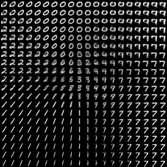
An example application

As an example application, we train a variational autoencoder on the handwritten digits dataset MNIST. We use multilayer perceptrons with one hidden layer with 500 units for both the encoder (\(q_{\phi}\)) and decoder (\(p_{\theta}\)) networks. Because we are interested in visualizing the latent space, we set the number of latent dimensions to 2. We use 1 sample per datapoint (\(L=1\)) and 100 datapoints per minibatch (\(M=100\)). We use stochastic gradient-ascent with a learning rate of 0.001 and train for 500 epochs (i.e., 500 passes over the whole dataset). The implementation can be seen online at https://github.com/gokererdogan/DeepLearning/tree/master/variational_autoencoder. We provide two implementations, one in pure theano and one in lasagne. We plot the latent space by varying the latent \(z\) along each of the two dimensions and sampling from the learned generative model. We see that the model is able to capture some interesting structure in the set of handwritten digits (compare to Fig4b in the original paper¹).

Appendix

Estimating \(\nabla_{\phi} \mathbb{E}_{q_{\phi}}[f(z)]\)

One common approach to estimating the gradient of such expectations is to make use of the identity \(\nabla_{\phi}q_{\phi} = q_{\phi} \nabla_{\phi} \log q_{\phi}\)

This estimator is known by various names in the literature from the REINFORCE algorithm to score function estimator or likelihood ratio trick. Given samples \(z^{(l)}, l=1\dots L\) from \(q_{\phi}(z|x)\), we can form an unbiased Monte Carlo estimate of the gradient of \(\mathcal{L}(\theta, \phi)\) with respect to \(\phi\) using this estimator. However, in practice it exhibits too high variance to be useful.

Bibliography